DS&A

How Fast is Your Algorithm?

Efficiency is important; people don’t like waiting for computers to slowly do things that ought to be fast.

So far we’ve been thinking about this in vague terms; we know, for example:

• Getting from an array-list is faster than from a linked list,
• Binary search is faster than linear search,
• Merge sort is faster than selection sort.

Now it’s time to go into detail: how do we know how fast an algorithm is?

An analogy

In the real world, there’s an obvious way to find out how long something takes: do it, and measure the time with a stopwatch.

Try using this stopwatch to measure how long the “1 + 1” model takes to finish.

Of course, computing 1 + 1 doesn’t realistically take this long; computers are too fast to measure manually with a stopwatch. This is just an analogy; really, we would make the computer start the timer, run the algorithm and stop the timer all automatically.

But this analogy does demonstrate some relevant issues:

• Neither you, nor the computer, can do two things at exactly the same time.(1) The measurement includes the time between starting the stopwatch and starting the computation.
• If you repeat the measurement, you might get a different result.
• Measuring the time for 1 + 1 doesn’t necessarily tell us how fast the same algorithm would be with different inputs; would 2 + 2 be twice as slow, four times as slow, or the same speed?

So, when we measure how long an algorithm takes to run, we should:

• Avoid doing anything else while the timer is running — for example, if the algorithm takes a list as input, create the list before starting the timer.
• Measure repeatedly and take an average.
• Try different inputs to see what factors affect the running time.

Let’s illustrate all of these points by measuring the insertion sort algorithm. To follow along, you’ll need the code for it.

The rest of the models on this page are real — they genuinely run the insertion sort algorithm in your browser, and measure the running time. This is called dynamic analysis, because we’re analysing the algorithm by actually running it.(2)

Timing a function

Let’s generate a list of 100 random numbers, and see how long it takes the insertion sort algorithm to sort this list.

We’ll use the perf_counter function from Python’s built-in time library. The running time of the insertion_sort function is the end time minus the start time. We’ll multiply by 1000 to measure in milliseconds instead of seconds.

from random import random
from time import perf_counter

def generate_random_list(n):
    lst = []
    for i in range(n):
        lst.append(random())
    return lst

def time_insertion_sort(n):
    # generate random list
    lst = generate_random_list(n)
    
    # measure running time
    start_time = perf_counter()
    insertion_sort(lst)
    end_time = perf_counter()
    
    # return time in milliseconds
    return 1000 * (end_time - start_time)

t = time_insertion_sort(100)
print('Time:', t, 'ms')

Try it out:

Taking an average

If we repeat the measurement, we don’t always get the same result. This isn’t just because the list is random — the clock itself is not perfectly accurate. The clock error will be small, but so are the times we’re measuring.

To get a more accurate measurement, we can execute the insertion sort algorithm repeatedly, and divide the total time by the number of repetitions to get an average. For example, let’s do 500 repetitions.

To do this properly, we should generate 500 different lists.(3)

def time_insertion_sort(n, repetitions):
    # generate random lists
    lists = []
    for i in range(repetitions):
        lst = generate_random_list(n)
        lists.append(lst)
    
    # measure running time
    start_time = perf_counter()
    for lst in lists:
        insertion_sort(lst)
    end_time = perf_counter()
    
    # return average in milliseconds
    return 1000 * (end_time - start_time) / repetitions

t = time_insertion_sort(100, 500)
print('Average time:', t, 'ms')

Try it out:

Trying different input sizes

The amount of input data usually has a big effect on how long an algorithm takes to run; so we should try lists of many different lengths. We’ll try lists of length 100, 200, 300, 400, and so on up to 2000.

This code will measure the average time for each length, and print the results in a tab-separated format.

def vary_list_length(max_n, step_size, repetitions):
    # print headers, tab-separated
    print('n', 'average time (ms)', sep='\t')
    
    for n in range(0, max_n+1, step_size):
        t = time_insertion_sort(n, repetitions)
        # print results, tab-separated
        print(n, t, sep='\t')

# try n = 100, 200, ..., 2000 with 200 repetitions each
vary_list_length(2000, 100, 200)

Try it out. It will take some time to run; reduce the number of repetitions if it’s too slow.

This data is easy to import into a spreadsheet, so we can plot a chart of the average running times:

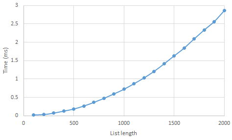
If you’re following along in Python, then your measurements may be quite different, but your chart should have a similar curved shape.

In particular, the chart is not a straight line — when the list is twice as long, insertion sort is not simply twice as slow; in this experiment, it was about four times as slow.

More input variations

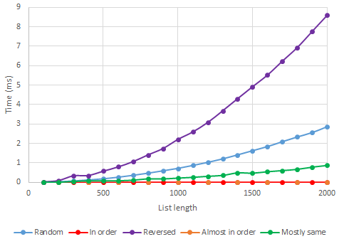
We can learn more about how efficient insertion sort is by trying different kinds of inputs — not just different list lengths. Real data usually isn’t completely random, so it could be useful to see whether the running time is affected by how disordered the input list is. We could try:

• Lists which are already in order, like [1, 2, 3, 4, 5].
• Lists which are completely out of order, like [5, 4, 3, 2, 1].
• Lists which are almost in order, like [1, 3, 4, 2, 5].
• Lists where most of the values are the same, like [1, 1, 1, 3, 1].

You can try out these options with the model below. If you’re following along in Python, you’ll need to change the generate_random_list function.

Putting these all together shows that the kind of input really makes a big difference to how fast the algorithm is:

Footnotes

1. CPUs with multiple cores can execute multiple instructions at once, but it is practically impossible to guarantee that two particular instructions will be exactly simultaneous.
2. Technically, we’re analysing an implementation of the algorithm; an alternative implementation of the same algorithm, e.g. in a different programming language, could give different results.
3. This isn’t just because an average over different inputs is more reliable. The algorithm is in-place, so if we used the same list 500 times, it would only be unsorted for the first run.

• Tags: 
• efficiency, dynamic analysis, algorithms