DS&A - Data Structures & Algorithms

‘Big O’ Notation

May 072018

By making a series of assumptions and considering only “large” inputs, we can analyse how efficient an algorithm is without actually running it. The result of this analysis is a mathematical formula called the complexity (or time complexity) of the algorithm. For example, we derived the formula n² for the selection sort algorithm.

Using standard notation, we would say that selection sort’s complexity is O(n²), or that selection sort is an O(n²) algorithm.

This formula says, very roughly, how much “work” the algorithm has to do as a function of n, which represents the “input size”. In this post, we’ll see how to make sense of this formula, and how to derive it with as little algebra as possible.

Complexity and running time

Before we begin, we should ask: is this even a useful kind of analysis? Perhaps surprisingly, after all the assumptions and approximations, this n² formula does say something useful about selection sort.

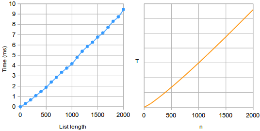
The chart on the left shows running times for selection sort, measured by actually running it. On the right is simply a plot of the equation T = n².

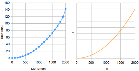
This is remarkably accurate, except the scales are completely different — the running times scale from 0 to 160 ms, while the complexity scales from 0 to 4 million. The scale on the right has no real meaning; the scale on the left measures real time, but this would be different on different computers or in different programming languages anyway.(1)

This is not a fluke. Here are running times for the linear search algorithm,(2) with its complexity function T = n plotted on the right:

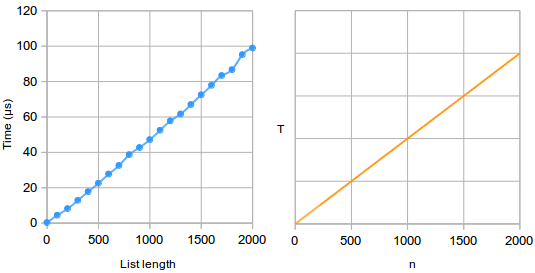
The complexity function still gives a fairly accurate estimate of how the running time depends on n.

Here are running times for binary search, alongside its complexity function T = log n on the right:

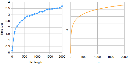
Again, the complexity function is fairly accurate except for scale.

‘Big O’ notation

The complexity gives a pretty accurate estimate of running time, but with no sense of scale. This is because we justified our simplifications and approximations by saying it would still be “roughly proportional” to the running time.

If the complexity is n² then the real running time might be approximately n², or 5n², or 100n²; these functions all have the same “shape” but different scales.(3)

To make it clear that we don’t know the scale, we use the capital letter O to mean “roughly proportional to”.(4) For example, when we say selection sort’s complexity is O(n²), this means its running time is roughly proportional to n².

There are many possible complexity functions, but some are very common. The following are in order from most efficient to least efficient.

O(1)

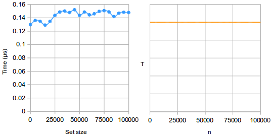
An algorithm’s complexity is O(1) if its running time doesn’t depend on the input size at all. This means that on average, the algorithm performs some fixed number of basic operations, whatever the input is.

An O(1) algorithm is called constant time, because there is a fixed constant amount of time it takes on average, regardless of n. For example, here are running times for the contains operation on Python’s built-in set data structure:

Every basic operation is O(1) by definition. Others include:

Get and set on an array.
Get, set and append* on an array-list.
Insert and remove at the start of a linked list.
Get, set*, remove* and contains-key on a hash map.
Insert*, remove* and contains on a hash set data structure.

The operations marked * are O(1) on average, but sometimes require copying every element to a new array, which is O(n).

O(log n)

The logarithm of a number is, roughly, how many times you can divide it by a given base before you get to 1.(5) This is relevant to divide and conquer algorithms, because it determines how many “divide” steps there are. The logarithm of n is written as log n.

If the complexity of an algorithm is O(log n), then we call it logarithmic time. Larger inputs will take more time, but not proportionally — for example, binary search only takes one more iteration for a list of length 200 than for a list of length 100.

O(log n) algorithms include:

Binary search.
Contains, insert and remove on a binary search tree.
Get, set, insert and remove on a skip list.
Poll from a binary heap priority queue.

O(n)

If the complexity of an algorithm is O(n) then the running time is roughly proportional to the input size. If the input is twice as large, the algorithm will take about twice as much time. This is called linear time.

Algorithms usually have linear complexity because they do a fixed amount of “work” for each item in some collection. Examples include:

Linear search.
Finding the minimum value, maximum value or sum of a list.
Insert and remove on an array-list.
Get, set, insert and remove on a linked list.
The “merge” procedure in the merge sort algorithm.

O(n log n)

A complexity of O(n log n) is common for efficient sorting algorithms, or other algorithms which take advantage of sorting, such as sweep line algorithms in geometry.(6) For example, here are running times for merge sort:

It’s hard to visually tell that this is not a straight line, but for larger n the curve is steeper. Therefore, for large enough n the algorithm will be slower than any linear complexity algorithm.

Algorithms with O(n log n) complexity include:

Merge sort, quicksort and heap sort.
The fast Fourier transform used in audio and image processing.
The monotone chain algorithm for finding convex hulls.

O(n²)

An algorithm is O(n²), or quadratic time, if the running time is roughly proportional to n². This is usually because of a “loop in a loop”; the algorithm has an inner loop which is O(n), and an outer loop which runs the inner loop n times, doing a total of n × n or n² basic operations.

Quadratic complexity is common for problems where simply iterating over a collection isn’t enough, such as sorting. Selection sort, insertion sort and bubble sort are all O(n²).

Also, many naive algorithms are O(n²) because they use an O(n) operation on a data structure, when a different data structure would do the same operation in constant time.

Comparing algorithms

The common complexities above are in order from most efficient to least efficient. To decide between two algorithms, we can often just go by complexity:

Merge sort is O(n log n), while selection sort is O(n²) — so merge sort is faster.
Getting from an array-list is O(1), but from a linked list it’s O(n) — so getting from an array-list is faster.

These conclusions are correct, at least assuming n is large enough for this analysis to be valid. It’s also a lot easier than doing a dynamic analysis for both algorithms, since we don’t have to try lots of inputs, avoid measurement errors, or run every algorithm on the same computer to get comparable results.

On the other hand, when two algorithms have the same complexity, we can’t decide between them so easily — for example, selection sort and insertion sort are both O(n²) — so we would do dynamic analysis to see which is faster.

Deriving the complexity of an algorithm

In the previous post we derived an exact formula for how many comparisons selection sort would do, and then made approximations to get the formula n². This took a fair bit of algebra, but using some simple rules it’s possible to derive the complexity much more easily.

Start with the code:

def selection_sort(lst):
    n = len(lst)
    for i in range(n):
        min_index = i
        for j in range(i+1, n):
            if lst[j] < lst[min_index]:
                min_index = j
        
        tmp = lst[i]
        lst[i] = lst[min_index]
        lst[min_index] = tmp

Any fixed sequence of basic operations is O(1), so we can simplify by writing how much “work” each part of the code takes:

def selection_sort(lst):
    # O(1)
    for i in range(n):
        # O(1)
        for j in range(i+1, n):
            # O(1)
        
        # O(1)

A loop multiplies the amount of “work” to be done. The outer loop iterates n times; the inner loop iterates over a range whose size is proportional to n.

def selection_sort(lst):
    # O(1)
    # O(n) times:
        # O(1)
        # O(n) times:
            # O(1)
        
        # O(1)

Simplifying:

def selection_sort(lst):
    # O(1)
    # O(n) times:
        # O(1)
        # O(n * 1) == O(n)
        # O(1)

O(n) is bigger than O(1), so the O(n) “dominates” the work inside the loop:

def selection_sort(lst):
    # O(1)
    # O(n) times:
        # O(n)